Introduction

Drug overdose (OD), defined as “when someone collapses, has blue skin, has convulsions, has difficulty breathing, loses consciousness, cannot be woken up, has a heart attach or dies while using drugs” (Bohnert, Tracy, & Galea, 2012), is being considered as an important public health issue. According the statistics from the CDC [2] more than 70,000 people died of drug OD in the US between 1999 and 2017. To better control and prevent the mortality and morbidity of drug OD, researchers [1] found that the drug OD morbidity among Hispanics and Black were significantly higher than Whites; [1] showed that age and socioeconomic characteristics may account for some, yet not all, the drug OD mortality and morbidity; [1] indicated that drug OD morbidity rate may vary at national, state and county levels.

Geographic approaches to drug OD death research have emerged in recent years. Researchers have demonstrated the drug OD morbidity was not equally distributed across different population subgroups [3,6] has also documented that the mortality and morbidity of drug OD varied geographically. For example, the mortality of drug OD in Hidalgo County, Texas was 4.8 per 100,000 residents in 2019, while this rate changed to 120.1 in Scioto County, Ohio for the same amount residents.

This study plans to explore the association between the number of drug OD inpatients with drug OD mortality and morbidity geospatially. This manuscript applies different Hierarchical models with various posterior assumptions. Conditional autoregressive (CAR) models with and without correlated/uncorrelated heterogeneity were utilized. To save the computation burden, this study just focused on the data of drug OD mortality and morbidity in Georgia state with the year of 2021.

This manuscript was arranged as follows: the models and the corresponding parameters assumptions were summarized in section 2. Model results were summarized in section 3. In section 4, conclusions and limitations were discussed

Methods

From the CDC website, the rate of death result from drug OD in Georgia State was 18 per 100,000, which ranked 18 among all other states in the US. One statistics showed from the Georgia Department of Public Health demonstrated that all drug OD deaths in Georgia increased by 55.9% from 2019 to 2021. Opioids, especially fentanyl, appear to be driving the increases (fentanyl-related OD deaths increased by 218.4%). To better understanding the story behind the highly increasing death rate caused by drug OD, it is important to check its association within the county-level data.

We first estimate the raw rates with Binomial assumption. Under this situation, the raw rate was computed as , where Yi and ni are the number of Drug morbidity and the total number of population in the i th county in George.

The second method we used was Hierarchical model with Binomial assumption. Under this situation, we assume the drug morbidity rate ϕi are independently and identically follows Beta(a,b), where we assume the a˜Gamma(1,0.0001) and b˜Gamma(1,0.0001).

The third method we used was Hierarchical model with Poisson assumption. Under this situation, we assume that Yi are conditionally independent follows Poi(ni ηi) given ηi . Assuming θi = log(ηi), we have θi follows the normal distribution with mean µ and variance σ2 ; both µ and σ2 were estimated by Monte Carlo Markov Chain (MCMC). This approach ignores spatial information about the counties. The model can also be written as θi = µ+vi, where µ and vi are overall mean and uncorrelated heterogeneity separately.

The fourth method we used was conditional autoregressive (CAR) model by adding only correlated heterogeneity. Under this situation, we consider as the precision, then our model could be assumed as [s1,s2,...sk] ˜ CAR − Normal(adj,num,τs),

where si is the correlated heterogeneity for the i^th county, num is the vector denote the number of neighbors of all n counties and adj denote the flat vector giving all adjacencies.

The last model we applied was conditional autoregressive (CAR) with both correlated and uncorrelated heterogeneity. Based on the 4th method we discussed, we added independent (uncorrelated) error terms (vi ). We have the following formula:

θⁱ = µ + vⁱ + sⁱ,

where µ, vⁱ and sⁱ are overall mean, uncorrelated heterogeneity and correlated heterogeneity.

As the 4^th model indicated, we have and as the precision for correlated heterogeneity and uncorrelated heterogeneity separately. We can write the model as:

[s¹,s²,,...,sⁿ] ˜ CAR − Normal(adj,num,τ^s)

[v¹,v²,,...,vⁿ] ˜ i.i.d N(0, τ^v).

The posteriors were estimated with MCMC with different number of burn-in and iterations.

The general model form for CAR with correlated and uncorrelated heterogeneity is θⁱ = β⁰ + β¹ Inpatientⁱ + vⁱ+ sⁱ.

Data source

The data was drawn from “Online analytically statistical information system (OASIS)”, tools for public health and public policy data analysis. This website was maintained by Georgia Department of Public Health. The drug OD morbidity data was selected for all the counties in Georgia with all the age ranges, all races and ethnicity, all educational background for male and female in 2021. The number of inpatients due to drug OD was also drawn by the same criteria.

Analysis

In this study, we used Bayesian technique to generate the model we mentioned above. As we all know, there are two main sources of information about the risk estimate for (θ) our prior beliefs, which is called prior distribution; and likelihood of observing the data given θ. We thus define some probability distribution of the risk estimate (θ), for example normal distribution or Poisson distribution. The posterior distribution is the result of combining the prior distribution and the likelihood, which could be used for drawing inferences.

Because our data may exist spatial autocorrelation, hierarchical models were applied in our analysis.

We summarized the 5 models mentioned above as follows: • Model 1: Raw data without any model assumption;

• Model 2: Yⁱ ˜ Bin(nⁱ,ϕⁱ) with ϕⁱ ˜ i.i.d Beta(a,b), where a and b were estimated using Bayesian inference without assuming spatial structure;

• Model 3: Yⁱ ˜ Poi(nⁱηⁱ) with ηⁱ ˜ i.i.d N(µ,σ₂), both µ and σ were unknown and could be estimated by MCMC without considering spatial county information, while adding uncorrelated heterogeneity information;

• Model 4: Yⁱ ˜ Poi(nⁱηⁱ) with θⁱ = log(ηⁱ) = µ + sⁱ where sⁱ ˜ CARNormal; for this model we account for the correlated heterogeneity imposed by the spatial structure;

• Model 5:Yⁱ ˜ Poⁱ(nⁱηⁱ) with θⁱ = log(ηⁱ) = µ + sⁱ where sⁱ + vⁱ, where sⁱ ˜ CAR−Normal(A,σs₂) and vi ˜ i.i.d N(0,σ₂); for this model we account for both correlated heterogeneity imposed by A and additional uncorrelated noise.

Additionally, Moran’s I statistic was used to measure the correlation coefficient for the overall spatial autocorrelation. The corresponding p-value and WAIC were also be discussed.

All the models mentioned above were generate using R (Version 4.2.1) with packages nimble, rCPP and INLA.

Results

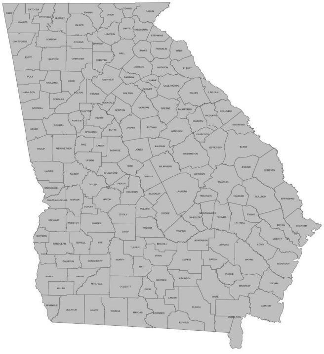
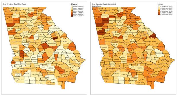
The Georgia state geographical map was shown in figure 1. The raw drug OD morbidity rate, which ranges from 0.01% to 0.07%, was shown in figure 2. Counties had the high drug OD morbidity rate such as Wilkinson county, Polk county, Glascock county and Lumpkin county, were located in the north part in Georgia. Counties such as Taylor, Dooly, Crisp, Irwin and Coffee had relatively low drug OD morbidity rate were located in central and south part in Georgia. Adjacent counties showed high correlated drug OD morbidity rate.

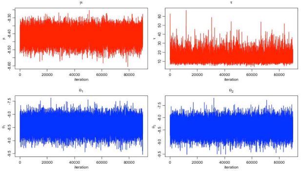
Figure 3 shows the MCMC estimation of µ, τ and σ with number of iteration 200000 times and the number of burn-in 30000 times. Both µ and τ showed a time-related trend. The estimated drug OD morbidity rate was around 0.02% with 95% HDI (0.017%, 0.035%), which was visuzlied in Figure 4. Figure 5 shows the comparison of Choropleth map of drug OD morbidity of raw rate and Bayesian hierarchical model. The estimated death rate with Bayesian hierarchical was ranged from 0.01% to 0.04%. Except Bulloch county and Thomas county remain the same death rate, the death rate in most counties were increased.

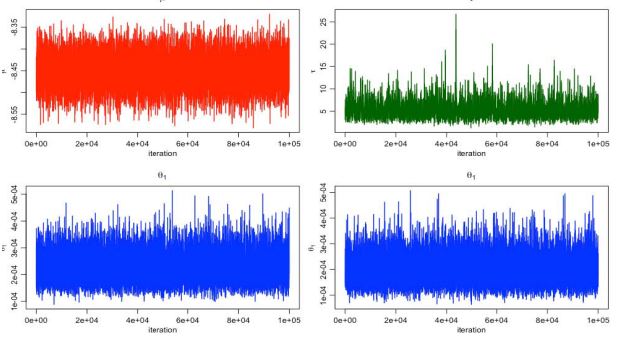
Figure 6 shows the the MCMC estimation of µ, τ, θ¹ and θ² with number of iteration 100000 times and the number of burn-in 10000 times. The plots indicate that the MCMC estimation may exist some time-related trend, without considering spatial structure.

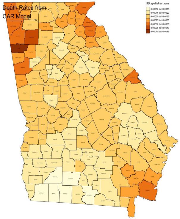
Figure 7 shows the the MCMC estimation of µ, τ, θ¹ and θ² with number of iteration 110000 times and the number of burnin 10000 times. After considering the spatial structure, the timerelated trend dismiss a lot. Figure 8 shows the estimated death after accounting for the correlated heterogeneity imposed by the spatial structure. The estimated death rate ranged from 0.01% to 0.045%. The relatively high drug OD morbidity rate were in southeast and northwest counties in Georgia.

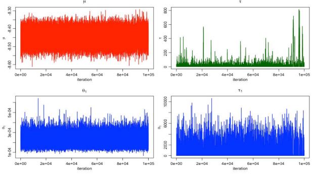
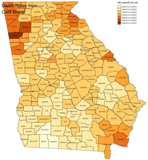
Figure 9 shows the the MCMC estimation of µ, τ, θ¹ and τ¹ with number of iteration 10100000 times and the number of burn-in 100000 times. After considering the spatial structure with both correlated and uncorrelated heterogeneity, the time-related trend dismiss a lot. Figure 10 shows the estimated death after accounting for the correlated and uncorrelated heterogeneity imposed by the spatial structure. The estimated death rate ranged from 0.01% to 0.045%. The relatively high drug OD morbidity rate were in southeast and northwest counties in Georgia, as model 4.

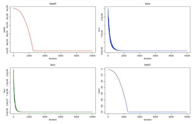
Figure 11 shows the estimation of β⁰ and β¹ , which are the estimated coefficient for the intercept and the estimated coefficient for the “Inpatient”. We can clearly see the negative association between number of inpatients and the drug OD morbidity rate.

Table 1 listed the Moran test for the model 5. As the p-value indicate, the drug OD morbidity rate being analyzed in our study was not randomly distributed in Georgia State.

Discussion

The United States is facing an epidemic of drug overdose. Using the Georgia “Online analytical statistical information system” mortality and morbidity data, this study focuses on drug overdose deaths, its spatial distribution across the Georgia state at the county level in the year of 2021, and its association with country level inpatient number. The study demonstrates that geographically association exist for drug OD morbidity in Georgia state, by using different spatial models. The raw data (without applying spatial techniques) indicates the high drug OD morbidity rate was not spatially correlated (Figure 2); while after using the spatial models, the high drug OD morbidity rate was common in southeast and northwest counties such as Camden county, Bartow county, Polk county and Carroll county.

This study also reveals that there is significant spatial autocorrelation among adjacent counties in the drug OD morbidity. Both traditional method and Bayesian techniques were used to check the spatial association. Both methods show similar patterns of spatial clustering across the county-level map in Georgia, though this spatial cluster differs at some levels. For example, the drug morbidity rate was ranged from 0-0.07% in original data, to 0-0.04% after applying the Bayesian spatial model. The high drug OD morbidity rate was randomly distributed in Georgia counties if only checking the raw death rate, while the spatial autocorrelation was shown after using the hierarchical Bayesian spatial model.

Furthermore, there is little difference in significant clusters for low drug OD morbidity rate between the model 2 and model 3, which methods didn’t account for the spatial county information. The Choropleth maps are similar in model 4 and model 5, which both methods considered the spatial autocorrelation. Because the empirical Bayesian hierarchical methods can correct for the rate where the data are too dispersed, the estimated death rates for model 4 and model 5 were more condensed than model 1 and model 2.

Presence of spatial autocorrelation in county level data in the drug OD morbidity rate is taken into consideration with the regression modeling. The correct model is specified to check the association between the number of inpatients and drug OD morbidity. The result was visualized in Figure 10 with Choropleth map. The estimation of the coefficients are shown in Figure 11. The results suggest that the drug OD morbidity rate is negatively associated with the number of inpatients. In other words, the drug OD morbidity could be prevented once the treatment get involved in time.

Though this article studies the drug OD morbidity geospatially with and without considering correlated/uncorrelated heterogeneity, there are some limitations. First of all, the number of baseline covariates was limited. The study was mainly focused on applying and checking different spatial models discussed in Dr. Rigdon’s class, hence I only checked the association between the drug OD morbidity and the number of inpatients. Future study should include more covariates to better understand what factors are closely related with drug OD morbidity. Secondly, the save the computation burden, I only consider the one state - Georgia. This may not correctly reflect the drug OD morbidity trend in the United States. Future study should consider more states. Thirdly, the current only used data collected in 2021, to fully understand the story, a wider time-range data should be applied.

References

1. Cano M. Racial/ethnic differences in US drug overdose mortality, 2017-2018. 2021a; 112.
2. Cano M. Racial/ethnic differences in US drug overdose mor- tality, 2017-2018. 2021b; 112: 2.
3. Cano M. Socioeconomic inequalities and Black/White disparities in US cocaine involved overdose mortality risk. 2022; 57.
4. Friedman JR, Hansen H. Evaluation of Increases in Drug Overdose Mortality Rates in the US by Race and Ethnicity Before and During the COVID-19 Pandemic. 2022; 79: 1.
5. Li G LB, Brandy JE. Prescription drug monitoring and drug overdose mortality. Inj Epidemiol. 2014.
6. Rossen LM, Khan D, Warner M. Hot spots in mortality from drug poisoning in the United States, 2007-2009. 2014; 26: 2.